Lagrange multipliers

$\newenvironment {prompt}{}{} \newcommand {\todo }[0]{} \newcommand {\oiint }[0]{{\large \bigcirc }\kern -1.56em\iint } \newcommand {\mooculus }[0]{\textsf {\textbf {MOOC}\textnormal {\textsf {ULUS}}}} \newcommand {\npnoround }[0]{\nprounddigits {-1}} \newcommand {\npnoroundexp }[0]{\nproundexpdigits {-1}} \newcommand {\npunitcommand }[1]{\ensuremath {\mathrm {#1}}} \newcommand {\RR }[0]{\mathbb R} \newcommand {\R }[0]{\mathbb R} \newcommand {\N }[0]{\mathbb N} \newcommand {\Z }[0]{\mathbb Z} \newcommand {\sagemath }[0]{\textsf {SageMath}} \newcommand {\d }[0]{\mathop {}\!d} \newcommand {\l }[0]{\ell } \newcommand {\ddx }[0]{\frac {d}{\d x}} \newcommand {\zeroOverZero }[0]{\ensuremath {\boldsymbol {\tfrac {0}{0}}}} \newcommand {\inftyOverInfty }[0]{\ensuremath {\boldsymbol {\tfrac {\infty }{\infty }}}} \newcommand {\zeroOverInfty }[0]{\ensuremath {\boldsymbol {\tfrac {0}{\infty }}}} \newcommand {\zeroTimesInfty }[0]{\ensuremath {\small \boldsymbol {0\cdot \infty }}} \newcommand {\inftyMinusInfty }[0]{\ensuremath {\small \boldsymbol {\infty -\infty }}} \newcommand {\oneToInfty }[0]{\ensuremath {\boldsymbol {1^\infty }}} \newcommand {\zeroToZero }[0]{\ensuremath {\boldsymbol {0^0}}} \newcommand {\inftyToZero }[0]{\ensuremath {\boldsymbol {\infty ^0}}} \newcommand {\numOverZero }[0]{\ensuremath {\boldsymbol {\tfrac {\#}{0}}}} \newcommand {\dfn }[0]{\textbf } \newcommand {\unit }[0]{\mathop {}\!\mathrm } \newcommand {\eval }[1]{\bigg [ #1 \bigg ]} \newcommand {\seq }[1]{\left ( #1 \right )} \newcommand {\epsilon }[0]{\varepsilon } \newcommand {\phi }[0]{\varphi } \newcommand {\iff }[0]{\Leftrightarrow } \DeclareMathOperator {\arccot }{arccot} \DeclareMathOperator {\arcsec }{arcsec} \DeclareMathOperator {\arccsc }{arccsc} \DeclareMathOperator {\si }{Si} \DeclareMathOperator {\scal }{scal} \DeclareMathOperator {\sign }{sign} \newcommand {\arrowvec }[1]{{\overset {\rightharpoonup }{#1}}} \newcommand {\vec }[1]{{\overset {\boldsymbol {\rightharpoonup }}{\mathbf {#1}}}} \DeclareMathOperator {\proj }{\vec {proj}} \newcommand {\veci }[0]{{\boldsymbol {\hat {\imath }}}} \newcommand {\vecj }[0]{{\boldsymbol {\hat {\jmath }}}} \newcommand {\veck }[0]{{\boldsymbol {\hat {k}}}} \newcommand {\vecl }[0]{\vec {\boldsymbol {\l }}} \newcommand {\uvec }[1]{\mathbf {\hat {#1}}} \newcommand {\utan }[0]{\mathbf {\hat {t}}} \newcommand {\unormal }[0]{\mathbf {\hat {n}}} \newcommand {\ubinormal }[0]{\mathbf {\hat {b}}} \newcommand {\dotp }[0]{\bullet } \newcommand {\cross }[0]{\boldsymbol \times } \newcommand {\grad }[0]{\boldsymbol \nabla } \newcommand {\divergence }[0]{\grad \dotp } \newcommand {\curl }[0]{\grad \cross } \newcommand {\lto }[0]{\mathop {\longrightarrow \,}\limits } \newcommand {\bar }[0]{\overline } \newcommand {\surfaceColor }[0]{violet} \newcommand {\surfaceColorTwo }[0]{redyellow} \newcommand {\sliceColor }[0]{greenyellow} \newcommand {\vector }[1]{\left \langle #1\right \rangle } \newcommand {\sectionOutcomes }[0]{} \newcommand {\HyperFirstAtBeginDocument }[0]{\AtBeginDocument } \newcommand {\epstopdfsetup }[0]{\setkeys {ETE}} changed the theorem header of amsthm failed\MessageBreak }}} \newcommand {\GetTitleStringSetup }[0]{\setkeys {gettitlestring}} \newcommand {\Sectionformat }[2]{#1}$

We give a new method of finding extrema.

Throughout this course, we hope it has become apparent that when given a problem:

There is more than one way to solve it.

Previously, we were finding extrema of functions $F:\R ^n\to \R$ when constrained to some set $S$ .

Let $F(x,y) = x^2+3y^2-4x-6y+7$ and let $S$ the set $S = \{(x,y):x^2 + y^2 \le 1\}$ Discuss how to find the maximum and minimum values of $F$ on $S$ .

To do this we first find the critical points of $F$ , that is where the components of $\grad F(x,y)$ are zero or do not exist. If these points are in $S$ , they become candidates for the maxima and minima.

Next we investigate the boundary of $S$ . To do this we must parameterize the boundary of $S$ , or express the boundary either in terms of $x$ or $y$ . In this case, we can express the boundary parametrically as $\vec {p}(t) = \vector {\cos (t),\sin (t)},$ or we could set $y = \pm \answer [given]{\sqrt {1-x^2}},$ or even $x = \pm \answer [given]{\sqrt {1-y^2}}.$ At this point we look for critical points on the boundary. These are also candidates for the extrema. Finally if the set has “corners,” we must also consider these as candidates for the extrema.

Above we see that a crucial step in computing extrema when constrained to a set is finding an explicit formula for the boundary. This could be very difficult or even impossible! If our constraining set had been $S = \{(x,y): x+y+\sin (xy) =0\}$ our previous method will not work, as we (at least this author!) cannot find an explicit formula describing the boundary (which in this case is the set) of the set above. Nevertheless, there is another way. It is called the method of Lagrange multipliers. This method is named after the mathematician Joesph-Louis Lagrange, which he first employed. This method relies on the gradient vector. Recall facts about the gradient vector:

$\grad F = \vector {\pp [F]{x_1},\pp [F]{x_2},\dots ,\pp [F]{x_n}}$ .
$\grad F(\vec {x})$ points in the direction that one must leave $\vec {x}$ in order to see the initial greatest increase in $F$ .
$\grad F(\vec {x})$ points in the direction that is perpendicular to any level surface of $F$ .

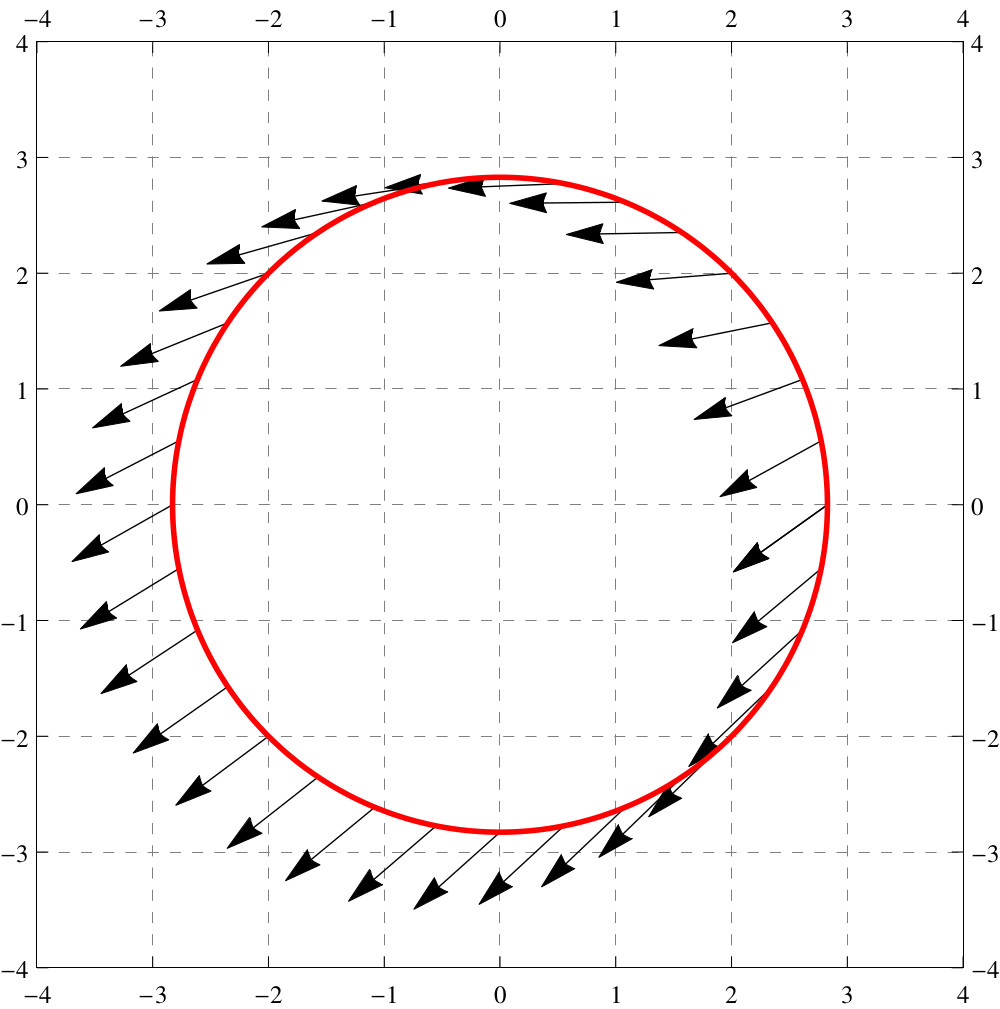
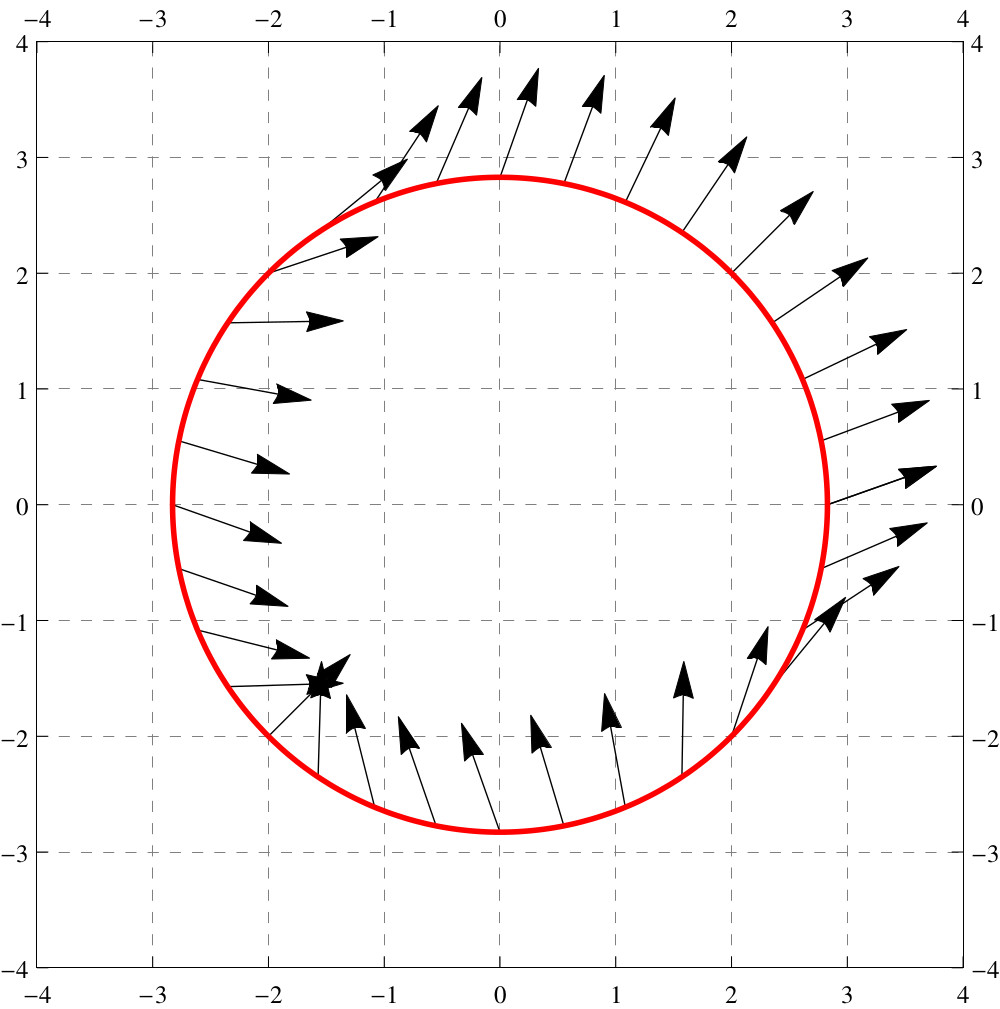
It is this last fact that we will look at now. Below we see level curves for some function $F:\R ^2\to \R$ along with a constraining curve that we will call $S$ :

Let’s add vectors to our graph that point in the direction of $\grad F(x,y)$ . We can do this without computation, since we understand the geometry of the gradient vector, the gradient vector is perpendicular to level curves:

Now we can observe something interesting: If for some point $(x,y)$ the gradient $\grad F(x,y)$ points in the “general” direction of the tangent vectors of $S$ , then $(x,y)$ cannot give an extremal value of $F$ , as moving along $S$ will either increase or decrease the value of $F$ . Here’s the upshot:

The only candidates for local extrema occur when the gradient of $F$ is perpendicular to $S$ .

How do we find these points? To do this, we will imagine that $S$ is a level curve for some other function $G:\R ^2\to \R$ , and define $S$ as: $S = \{(x,y):G(x,y)= c\}$ now, the candidates for extrema of $F$ when constrained to a curve $S$ are found by finding $(x,y)$ such that $\grad F(x,y) = \lambda \cdot \grad G(x,y)$ since $(x,y)$ that satisfy this equation are those where the gradient vectors of $F$ are perpendicular to the level curve $G(x,y)= c$ . This is the essence of the method of Lagrange multipliers.

Lagrange Multipliers Let $F:\R ^n\to \R$ , $G:\R ^n\to \R$ , $\grad G(\vec {x}) \ne \vec {0}$ , and let $S$ be the level set $S = \{\vec {x}: G(\vec {x}) = c\}$ If $F$ has extrema when constrained to $S$ at $\vec {x}$ , then $\grad F(\vec {x}) = \lambda \cdot \grad G(\vec {x})$ for some number $\lambda$ .

Working with geometry

Lagrange multipliers tell us that to maximize a function $F:\R ^2\to \R$ along a curve defined by $G(x,y) = c$ , we need to find where $\grad F$ is perpendicular to $G$ . In essence we are detecting geometric behavior using the tools of calculus.

Below we have plotted a curve $G(x,y) = c$ along with $\grad F$ .

Find the candidates for the maximum and minimum values for $F$ when restricted to $G(x,y) = c$ .

At the candidates for the extrema, we know that the gradient vector of $F$ must be parallelperpendicular to the curve $G(x,y) = c$ . Hence we see that the points $(x,y)\approx (\answer [given,tolerance=.3]{2.5},\answer [given,tolerance=.5]{.9})$ and $(x,y)\approx (-2.3,\answer [given,tolerance=.3]{-1.7})$ are our candidates for extrema.

Below we have plotted a curve $G(x,y) = c$ along with $\grad F$ .

Find the candidates for the maximum and minimum values for $F$ when restricted to $G(x,y) = c$ .

At the candidates for the extrema, we know that the gradient vector of $F$ must be parallelperpendicular to the curve $G(x,y) = c$ . Hence we see that the points $\begin{align*} (x,y) &= (\answer[given]{2},2)\\ (x,y) &= (-2,\answer[given]{-2})\\ (x,y) &\approx (\answer[given,tolerance=.3]{0.8},-2.7)\\ (x,y) &\approx (-2.7,\answer[given,tolerance=.3]{0.8}) \end{align*}$ are our candidates for extrema.

Working with algebra

Let’s work an example.

Let $F(x,y,z) = (1+x^2)(1+y^2)(1+z^2)$ and let $S$ the set: $S = \{(x,y):x+y+z=1,\text { where }x\ge 0, y\ge 0,z\ge 0\}$ Find the absolute maximum and minimum values of $F$ on $S$ . This problem was a problem posed in the April $2004$ issue of Math Horizons:

We’ll check the critical points of $F$ . First compute $\grad F$ : $\grad F(x,y,z) = \begin {bmatrix} \answer [given]{2x(1+y^2)(1+z^2)}\\ \answer [given]{2y(1+x^2)(1+z^2)}\\ \answer [given]{2z(1+x^2)(1+y^2)} \end {bmatrix}$ From this we see $\grad F = \vec {0}$ when $\begin{align*} x &= \answer[given]{0}\\ y &= \answer[given]{0}\\ z &= \answer[given]{0}. \end{align*}$ Now we need to check along the boundary of $S$ . Note that $S$ is a tetrahedron with vertices at $(1,0,0)$ , $(0,1,0)$ and $(0,0,1)$ . In particular, since the boundary is not differentiable at the vertices of $S$ , we must check the point $(1,0,0)$ , $(0,1,0)$ , and $(0,0,1)$ . At each of these points, the value of $F$ is $\answer [given]{2}$ .

Using Lagrange multipliers, we will check all other points on $S$ by setting $G(x,y,z) = x+y+z$ and computing $\grad G$ : $\grad G(x,y,z) = \vector {\answer [given]{1},\answer [given]{1},\answer [given]{1}}$ We need to find points $(x,y,z)$ such that $\grad F(x,y,z) = \lambda \cdot \grad G(x,y,z)$ for some number $\lambda$ . Write with me

$\begin{align*} 2x(1+y^2)(1+z^2) &=\lambda \cdot 1\\ 2y(1+x^2)(1+z^2) &=\lambda \cdot 1\\ 2z(1+x^2)(1+y^2) &=\lambda \cdot 1 \end{align*}$ and $x+y+z=1.$ Note the symmetry of the components of $\grad F$ . From this we see that $x = y = z.$ Hence $\begin{align*} x+y+z&=1\\ \answer[given]{3}x &= 1\\ x &= \answer[given]{1/3}. \end{align*}$ Thus to find extrema for $F$ when restricted to $S$ , we check the value of $F$ at the points above. Write with me $\begin{align*} F(1,0,0) &= \answer[given]{2}\\ F(0,1,0) &= \answer[given]{2}\\ F(0,0,1) &= \answer[given]{2}\\ F(1/3,1/3,1/3) &= \answer[given]{1000/729} \end{align*}$ We now see, via the Extreme Value Theorem, that the absolute minimum of $F$ when restricted to $S$ is given by $(x,y,z) = (\answer [given]{1/3},\answer [given]{1/3},\answer [given]{1/3})$ and the absolute maximums are at the points $(1,0,0)$ , $(0,1,0)$ , and $(0,0,1)$ .

The Lagrangian

Finally, we should point our that there are other ways to view Lagrange multipliers.

Given functions $F:\R ^n\to \R$ and $G:\R ^n\to \R$ the Lagrangian is the function $\mathcal {L}(\vec {x},\lambda ) = F(\vec {x}) - \lambda \cdot G(\vec {x}).$

Thus to check whether $\grad F(\vec {x}) = \lambda \cdot \grad G(\vec {x})$ is equivalent to checking where $\grad \mathcal {L}(\vec {x},\lambda ) = \vec {0}$ or has undefined components. When working with constrained optimization problems by hand, the Lagrangian doesn’t help much, since your next step is to look at $\grad \mathcal {L}(\vec {x},\lambda ) = \vec {0}.$ However, there are certain advantages to working with the Lagrangian:

If you are working with a computer, it might be better to work in terms of the Lagrangian, as there are efficient algorithms for checking when the gradient of the function is zero.
Working with the Lagrangian gives a method for changing “constrained” optimization to “unconstrained” optimization, as we are simply finding the critical points of $\mathcal {L}(\vec {x},\lambda )$ .
The Lagrangian shows us a symmetry between $F$ and $G$ .

For some interesting extra reading check out: