Functions of several variables

$\newenvironment {prompt}{}{} \newcommand {\todo }[0]{} \newcommand {\oiint }[0]{{\large \bigcirc }\kern -1.56em\iint } \newcommand {\mooculus }[0]{\textsf {\textbf {MOOC}\textnormal {\textsf {ULUS}}}} \newcommand {\npnoround }[0]{\nprounddigits {-1}} \newcommand {\npnoroundexp }[0]{\nproundexpdigits {-1}} \newcommand {\npunitcommand }[1]{\ensuremath {\mathrm {#1}}} \newcommand {\RR }[0]{\mathbb R} \newcommand {\R }[0]{\mathbb R} \newcommand {\N }[0]{\mathbb N} \newcommand {\Z }[0]{\mathbb Z} \newcommand {\sagemath }[0]{\textsf {SageMath}} \newcommand {\d }[0]{\mathop {}\!d} \newcommand {\l }[0]{\ell } \newcommand {\ddx }[0]{\frac {d}{\d x}} \newcommand {\zeroOverZero }[0]{\ensuremath {\boldsymbol {\tfrac {0}{0}}}} \newcommand {\inftyOverInfty }[0]{\ensuremath {\boldsymbol {\tfrac {\infty }{\infty }}}} \newcommand {\zeroOverInfty }[0]{\ensuremath {\boldsymbol {\tfrac {0}{\infty }}}} \newcommand {\zeroTimesInfty }[0]{\ensuremath {\small \boldsymbol {0\cdot \infty }}} \newcommand {\inftyMinusInfty }[0]{\ensuremath {\small \boldsymbol {\infty -\infty }}} \newcommand {\oneToInfty }[0]{\ensuremath {\boldsymbol {1^\infty }}} \newcommand {\zeroToZero }[0]{\ensuremath {\boldsymbol {0^0}}} \newcommand {\inftyToZero }[0]{\ensuremath {\boldsymbol {\infty ^0}}} \newcommand {\numOverZero }[0]{\ensuremath {\boldsymbol {\tfrac {\#}{0}}}} \newcommand {\dfn }[0]{\textbf } \newcommand {\unit }[0]{\mathop {}\!\mathrm } \newcommand {\eval }[1]{\bigg [ #1 \bigg ]} \newcommand {\seq }[1]{\left ( #1 \right )} \newcommand {\epsilon }[0]{\varepsilon } \newcommand {\phi }[0]{\varphi } \newcommand {\iff }[0]{\Leftrightarrow } \DeclareMathOperator {\arccot }{arccot} \DeclareMathOperator {\arcsec }{arcsec} \DeclareMathOperator {\arccsc }{arccsc} \DeclareMathOperator {\si }{Si} \DeclareMathOperator {\scal }{scal} \DeclareMathOperator {\sign }{sign} \newcommand {\arrowvec }[1]{{\overset {\rightharpoonup }{#1}}} \newcommand {\vec }[1]{{\overset {\boldsymbol {\rightharpoonup }}{\mathbf {#1}}}} \DeclareMathOperator {\proj }{\vec {proj}} \newcommand {\veci }[0]{{\boldsymbol {\hat {\imath }}}} \newcommand {\vecj }[0]{{\boldsymbol {\hat {\jmath }}}} \newcommand {\veck }[0]{{\boldsymbol {\hat {k}}}} \newcommand {\vecl }[0]{\vec {\boldsymbol {\l }}} \newcommand {\uvec }[1]{\mathbf {\hat {#1}}} \newcommand {\utan }[0]{\mathbf {\hat {t}}} \newcommand {\unormal }[0]{\mathbf {\hat {n}}} \newcommand {\ubinormal }[0]{\mathbf {\hat {b}}} \newcommand {\dotp }[0]{\bullet } \newcommand {\cross }[0]{\boldsymbol \times } \newcommand {\grad }[0]{\boldsymbol \nabla } \newcommand {\divergence }[0]{\grad \dotp } \newcommand {\curl }[0]{\grad \cross } \newcommand {\lto }[0]{\mathop {\longrightarrow \,}\limits } \newcommand {\bar }[0]{\overline } \newcommand {\surfaceColor }[0]{violet} \newcommand {\surfaceColorTwo }[0]{redyellow} \newcommand {\sliceColor }[0]{greenyellow} \newcommand {\vector }[1]{\left \langle #1\right \rangle } \newcommand {\sectionOutcomes }[0]{} \newcommand {\HyperFirstAtBeginDocument }[0]{\AtBeginDocument } \newcommand {\epstopdfsetup }[0]{\setkeys {ETE}} changed the theorem header of amsthm failed\MessageBreak }}} \newcommand {\GetTitleStringSetup }[0]{\setkeys {gettitlestring}} \newcommand {\Sectionformat }[2]{#1}$

We introduce functions that take vectors or points as inputs and output a number.

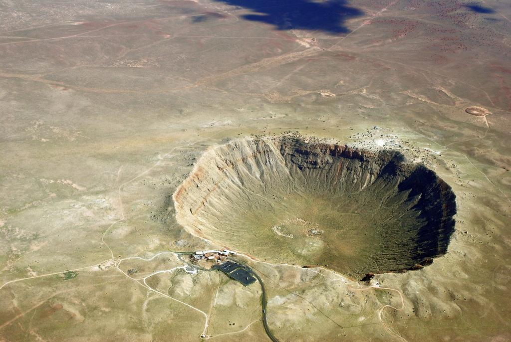
The world is constantly changing. Sometimes this change is very slow, other times it is shockingly fast. Consider Meteor Crater in northern Arizona:

This area was once grasslands and woodlands inhabited by bison, camels, wooly mammoths, and giant ground sloths. During the Pleistocene epoch, a meteor only $40$ meters in diameter collided with the Earth and this changed very quickly. The collision released around $4\times 10^{16}$ joules of energy, comparable to the energy released by a large nuclear weapon. A fireball extended out $10$ kilometers from the center of the impact, destroying all life in its wake. It is estimated it took one-hundred years for the local plant and animal life to repopulate the area. Fifty-thousand years later, the remains of the impact crater are still intact on our ever-changing Earth.

To help us understand events like these, we need to precisely describe what we are observing (in this case, the crater). To do this we use a contour map, often called a topographical map:

In essence we are looking at the crater from directly above, and each curve in the maps above represents a fixed, constant height. Mathematically, a contour map describes a function of two variables. We will now define a more general case of a function of $n$ variables. These are often called functions of several variables.

A function of several variables with domain $D$ is a relation $\begin{align*} F: D\subset \R^n &\to \R\\ \vec{x} &\mapsto y\\ \vector{x_1,x_2,\dots,x_n} &\mapsto y \end{align*}$ that assigns every ordered tuple in $D$ ( $D$ is a subset of $\R ^n$ ) a unique real number in $\R$ . The set of all outputs of $F$ is the range (a subset of $\R$ ).

Let’s investigate functions of two variables, $F:\R ^2\to \R$ :

Consider $F(x,y) = \sqrt {1-\frac {x^2}{9}-\frac {y^2}{4}},$ and compute $F(2,1)$ . $F(2,1) = \answer {\sqrt {11}/6}$

What is the domain of $F$ ? The domain is all vectors $\vector {x,y}$ allowable as inputoutput for $F$ . Because of the square-root, we need $\vector {x,y}$ such that: $0 \le \answer {1-\frac {x^2}{9}-\frac {y^2}{4}}$ Write $\begin{align*} 0&\le 1-\frac{x^2}{9}-\frac{y^2}{4}\\ \answer{\frac{x^2}{9}+\frac{y^2}{4}}&\le 1 \end{align*}$ This inequality describes the interior of an ellipse centered in the $(x,y)$ -plane.

What is the range of $F$ ? The range is the set of all possible inputoutput values. The square-root ensures that all output is $\geq \answer {0}$ . Since the $x$ and $y$ terms are squared, then subtracted, inside the square-root, the largest output value comes at $x=\answer {0}$ , $y=\answer {0}$ : $F(0,0) = \answer {1}$ . Thus the range $R$ is the interval $[\answer {0},\answer {1}]$ .

Now let’s ponder functions of three variables, $F:\R ^3\to \R$ .

Consider $F(x,y,z) = \frac {x^2+z+3\sin y}{x+2y-z},$ and compute $F(3,0,2)$ . $F(3,0,2)=\answer {11}$

What is the domain of $F$ ? The domain is all vectors $\vector {x,y,z}$ allowable as inputoutput for $F$ . Because of denominator in the expression representing $F$ , we need to find $\vector {x,y,z}$ such that $\answer {x+2y-z} \ne 0$ We recognize that the set of all points in $\R ^3$ that are not in $D$ form a lineplanecircle in space that passes through the origin, with normal vector $\vec {n} = \vector {\answer {1},\answer {2},\answer {-1}}$

What is the range of $F$ ? The range $R$ is the set of all possible inputoutput values. It happens to be all ofa proper subset of $\R$ . There is no set way of establishing this. Rather, to get numbers near $0$ we can let $y=0$ and choose $z \approx -x^2$ . To get numbers of arbitrarily large magnitude, we can let $z\approx x+2y$ .

Visualizing functions of several variables

The graph of a function of a single variable, $y=f(x)$ is a curve in a two-dimensional plane. The graph of a function of two variables, $z = F(x,y)$ is a surface in three-dimensional space. The graph of a function of three variables, $w=F(x,y,z)$ is a surface in four-dimensional space. How can we visualize such functions? While technology is readily available to help us graph functions of two variables, there is still a paper-and-pencil approach that is useful. This technique is know as sketching level sets. When working with functions $F:\R ^2\to \R$ , our level sets are level curves, and when working with functions $F:\R ^3\to \R$ , our level sets are level surfaces.

Level curves

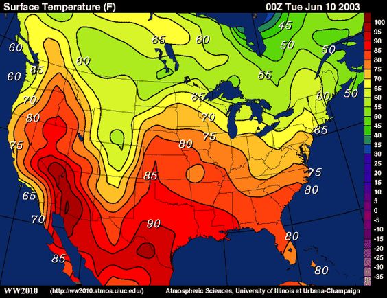
It may be surprising to find that the problem of representing a three dimensional surface on paper is familiar to most people (they just don’t realize it). Topographical maps, like the one shown in Figure represent the surface of Earth by indicating points with the same elevation with contour lines. Another example would be isotherms, we see these in weather maps:

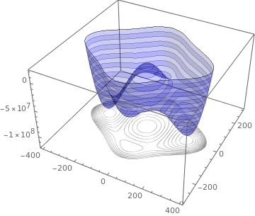
Given a function $z=F(x,y)$ , we can draw a “topographical map” of $F$ by drawing level curves (or, contour lines). A level curve at $z=c$ is a curve in the $(x,y)$ -plane such that for all points $(x,y)$ on the curve, $F(x,y) = c$ . Below we see a surface with level curves drawn beneath the surface:

When drawing level curves, it is important that the $c$ values are spaced equally apart as that gives the best insight to how quickly the “elevation” is changing. Examples will help one understand this concept.

Let $F(x,y) = \sqrt {1-\frac {x^2}{9}-\frac {y^2}{4}}$ . Find the level curves of $f$ for $c=0$ , $0.2$ , $0.4$ , $0.6$ , $0.8$ and $1$ .

Let’s work somewhat generally. Each of our level curves will be of the form $\begin{align*} c &= \sqrt{1-\frac{x^2}{9}-\frac{y^2}{4}}\\ c^2 &= \answer[given]{1-\frac{x^2}{9}-\frac{y^2}{4}}. \end{align*}$ Now we just need to plot each of the following implicit functions: $\begin{align*} 0^2 &= 1-\frac{x^2}{9}-\frac{y^2}{4}, \\ 0.2^2 &= 1-\frac{x^2}{9}-\frac{y^2}{4}, \\ 0.4^2 &= 1-\frac{x^2}{9}-\frac{y^2}{4}, \\ 0.6^2 &= 1-\frac{x^2}{9}-\frac{y^2}{4}, \\ 0.8^2 &= 1-\frac{x^2}{9}-\frac{y^2}{4}, \\ 1^2 &= 1-\frac{x^2}{9}-\frac{y^2}{4}. \end{align*}$ You can now plot these implicit functions with your favorite graphing device. As a gesture of friendship, we have included a graph of these level curves: $\graph [xmin=-5, xmax=5, ymin=-2.3, ymax=2.3]{0^2 = 1-\frac {x^2}{9}-\frac {y^2}{4}, 0.2^2 = 1-\frac {x^2}{9}-\frac {y^2}{4}, 0.4^2 = 1-\frac {x^2}{9}-\frac {y^2}{4},0.6^2 = 1-\frac {x^2}{9}-\frac {y^2}{4},0.8^2 = 1-\frac {x^2}{9}-\frac {y^2}{4},1^2 = 1-\frac {x^2}{9}-\frac {y^2}{4}}$ In the image below, the level curves are drawn on a graph of $F$ in space.

Note how the elevations are evenly spaced. Near the level curves of $c=0$ and $c=0.2$ we can see that $F$ indeed is growing quickly.

If one example is good, two is better.

Let $F(x,y) = \frac {x+y}{x^2+y^2+1}$ . Find the level curves for $z=c$ .

We begin by setting $F(x,y)=c$ for an arbitrary $c$ and seeing if algebraic manipulation of the equation reveals anything significant. $\begin{align*} \frac{x+y}{x^2+y^2+1} &= c \\ x+y &= \answer[given]{c(x^2+y^2+1)}. \end{align*}$ You may recognize this as a circle; regardless, plotting $x+y = c(x^2+y^2+1).$ for $c=0,\pm 0.2$ , $\pm 0.4$ , and $\pm 0.6$ will reveal the shape of the surface defined by $F$ . As a gesture of friendship, we have included a graph of these level curves: $\graph [xmin=-15, xmax=15, ymin=-7, ymax=7]{x+y = 0.6(x^2+y^2+1),x+y = 0.4(x^2+y^2+1), x+y = 0.2(x^2+y^2+1),x+y = 0,x+y = -0.2(x^2+y^2+1),x+y = -0.4(x^2+y^2+1),x+y = -0.6(x^2+y^2+1)}$

Seeing the level curves helps us understand the graph. For instance, the graph does not make it clear that one can “walk” along the line $y=-x$ without elevation change, though the level curve does.

Level surfaces

It is very difficult to produce a meaningful graph of a function of three variables.

A function of one variable can be visualized as a curve drawn in two dimensions.
A function of two variables can be visualized as a surface drawn in three dimensions.
A function of three variables can be visualized as a hypersurface drawn in four dimensions.

There are a few techniques one can employ to try to “picture” a graph of three variables. One is an analogue of level curves: level surfaces. Given $w=f(x,y,z)$ , the level surface at $w=c$ is the surface in space formed by all points $(x,y,z)$ where $f(x,y,z)=c$ . Time for an example.

If a point source $S$ is radiating energy, the intensity $I$ at a given point $P$ in space is inversely proportional to the square of the distance between $S$ and $P$ . That is, when $S=(0,0,0)$ , $\begin{align*} I(x,y,z) &= \frac{\text{some constant}}{\text{distance squared}}\\ &=\frac{k}{x^2+y^2+z^2} \end{align*}$ for some constant $k$ . Let $k=1$ ; find the level surfaces of $I$ .

We can (mostly) answer this question using “common sense.” If energy (say, in the form of light) is emanating from the origin, its intensity will be the same all a points equidistant from the origin. That is, at any point on the surface of a sphere centered at the origin, the intensity should be the same. Therefore, the level surfaces are spheres.

We now confirm this “common sense” mathematically. The level surface at $I=c$ is defined by $c = \frac {1}{x^2+y^2+z^2}.$ Algebra reveals $\answer [given]{x^2+y^2+z^2} = \frac {1}{c}.$ Given an intensity $c$ , the level surface $I=c$ is a sphere of radius $1/\sqrt {c}$ , centered at the origin. Every point on each sphere experiences the same intensity of the radiating energy. For your viewing pleasure, we present the level surface of this curve graphed by ?? Here $c$ is the intensity.

If the distance is doubled, is the intensity halved?

yes no

Experiment with how the level surface changes when the intensity is halved. We can see that that the closer one is to the source, the more rapidly the intensity changes.