Divergence measures the rate field vectors are expanding at a point.
The divergence of a vector field
Let’s state the definition:
Given a vector field , where the divergence is given by Some authors use the
notation for the divergence of a vector field.
Is the divergence of a vector field a scalar or a vector?
vector. scalar. neither a
vector nor a scalar.
The divergence is a number that tells you how much the field is expanding at a point.
However, no directional information is given.
What does divergence measure?
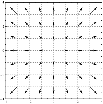
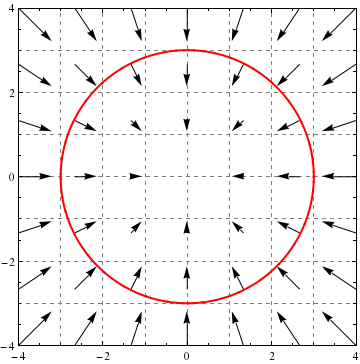
As we’ve already said, divergence measures the rate field vectors are expanding at a point. The most obvious example of a vector field with nonzero divergence is :
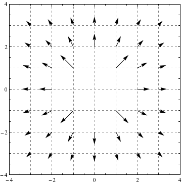
Now we will see a radial vector field with zero divergence.
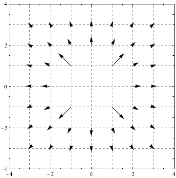
Now let’s see a radial vector field with negative divergence.
Measuring flow across a curve
Let be a vector field, be a smooth vector valued function tracing a curve exactly once as runs from to ,
Recall that the line integral measures the accumulated flow of a vector field along a curve. We see this because measures how “aligned” field vectors are with the direction of the path . On the other hand, if we set then for any given value of , is a vector that is orthogonal to . Moreover, given a closed curve, where is parameterized with the interior on the left, points outward. Below we see a curve along with some tangent vectors and some outward normal vectors :
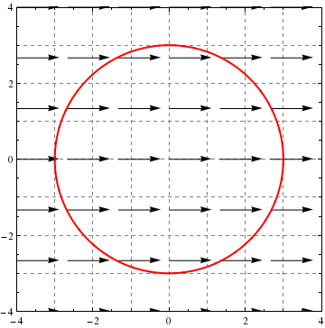
Consider the following vector field and curve parameterized by : 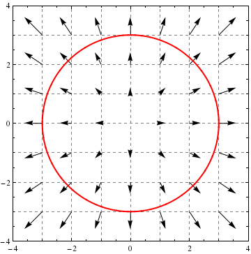 Do you expect to be positive, zero, or negative?
positive zero negative
With our next example, we’ll get our hands dirty.
Below we see a closed curve along with some representative field vectors of a vector
field :  Setting or (depending on the direction of the curve), estimate:
Connections to Green’s Theorem
Finally, note that if , then:
We also see that this leads us to the flux form of Green’s Theorem: